Kinematic loops
While preparing for my exams here is a post to just put some thoughts about kinematic loops in joints on paper. In this discussion I will first limit myself to the Kanes method, since that is currently the best supported method within SymPy. In this post I will start with a quick look on what are constraints. Next we will start forming some arbitrary kinematic loops, which would be good test cases. After which I hope to speak a bit about how the problems can be solved and some different kinds of possible implementations.
The table below shows the different definitions for the symbols used in this post.
| Symbol | Description |
|---|---|
| Arrow types | |
| Translation | |
 |
Rotation |
| Arrow colors | |
 |
Degree of Freedom (DoF) |
 |
Constrained DoF, DoF which has become dependent on other generalized coordinates |
 |
Active constraint |
 |
Already satisfied constraint, constraint that is already satisfied by another constraint from an earlier joint |
 |
Dependent constraint, two or more constraints from the same joint which are dependent on each other (ot all are active) |
| Joints | |
 |
PinJoint, a simple hinge with 1 DoF |
 |
PrismaticJoint, translational joint with 1 DoF |
 |
SphericalJoint, a rotational joint with 3 DoF |
What is a constraint?
In general, we talk about two kind of constraints, namely: holomic constraints and nonholonomic constraints. Holonomic constraints you can say are position constraints (i.e. constraints on the configuration), e.g. this point may not move in the x direction. Nonholomic constraints are velocity constraints that cannot be integrated to the configuration space. You can most of the time say of nonholonomic constraints that a point should move along this path. The most common nonholonomic constraint is seen in wheeled vehicles, which as you know cannot ride sideways, but have to stir to go right or left. In the currently implemented joints, namely the Pinjoint and the PrismaticJoint, only have holonomic constraints. Therefore I will mainly be discussing the holonomic constraints. If you by the way want to know more, here are two excellent pages about holonomic and nonholonomic constraints.
Now is of course the question: how do constraints precisely apply to joints?
Suppose we have two bodies, one is the ground and one is a free moving body. Which of course has 6 degrees of freedom (DoF). Introducing a PinJoint between the two bodies will give 5 constraints, leaving only one free variable. This is also visualized in the first two images below, where green arrows are DoF and the red are constraints.
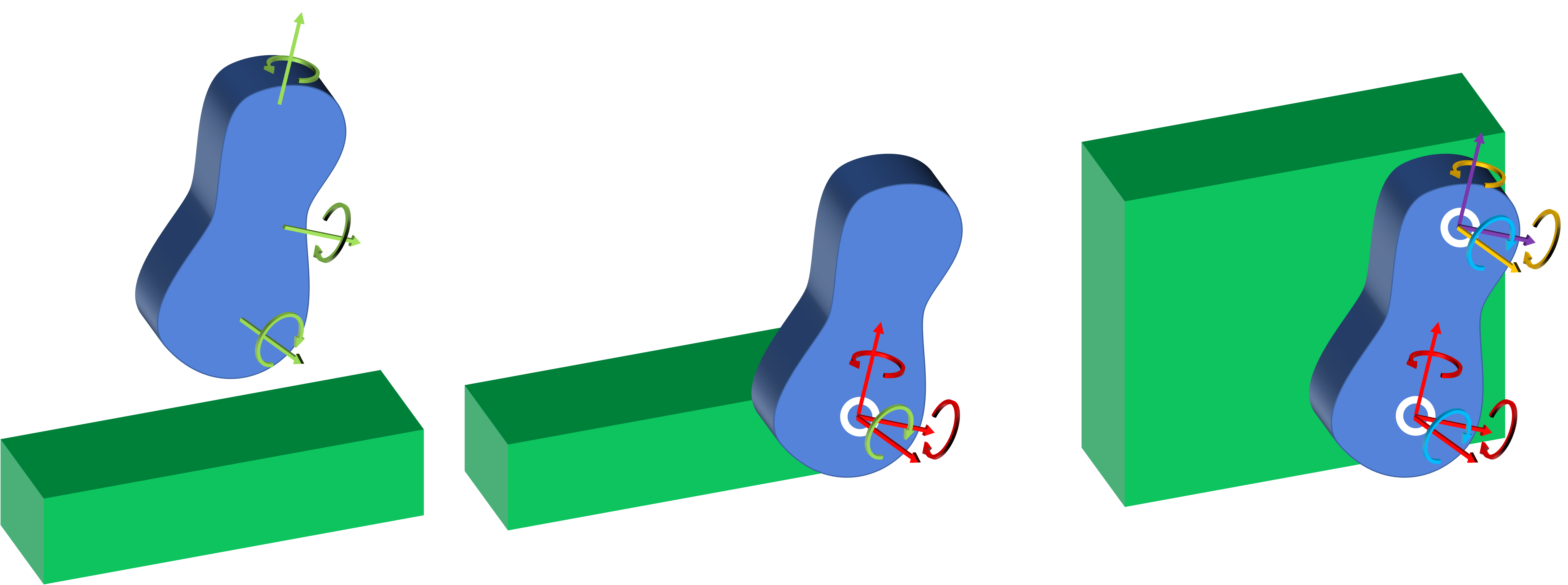
Of course this is not the way the PinJoint is implemented, rather than adding those 5 constraints, while having 6 generalized coordinates. It just uses one generalized coordinate. But this principle that you can also describe a joint in essence as constraints is important to keep in mind.
Now the above example is still quite simple, since there is no duplication in the constraints, but if you will actually get a loop, than you’ll start seeing that some constraints are duplicates. This is also shown in the last image above, where we add an extra PinJoint between the blue body and the ground using constraints. And as you can see is that we have multiple duplicate constraints (orange), which are constraints already satisfied by the constraints in the open loop joint. Besides those we also have two dependent constraints (purple) of which we only need to apply one. Note the DoF have become blue, meaning that they have become dependent DoF.
Test cases
So let’s list a few test cases:
| System | Joints | # open loop DoF | # active constraints | # closed loop DoF |
|---|---|---|---|---|
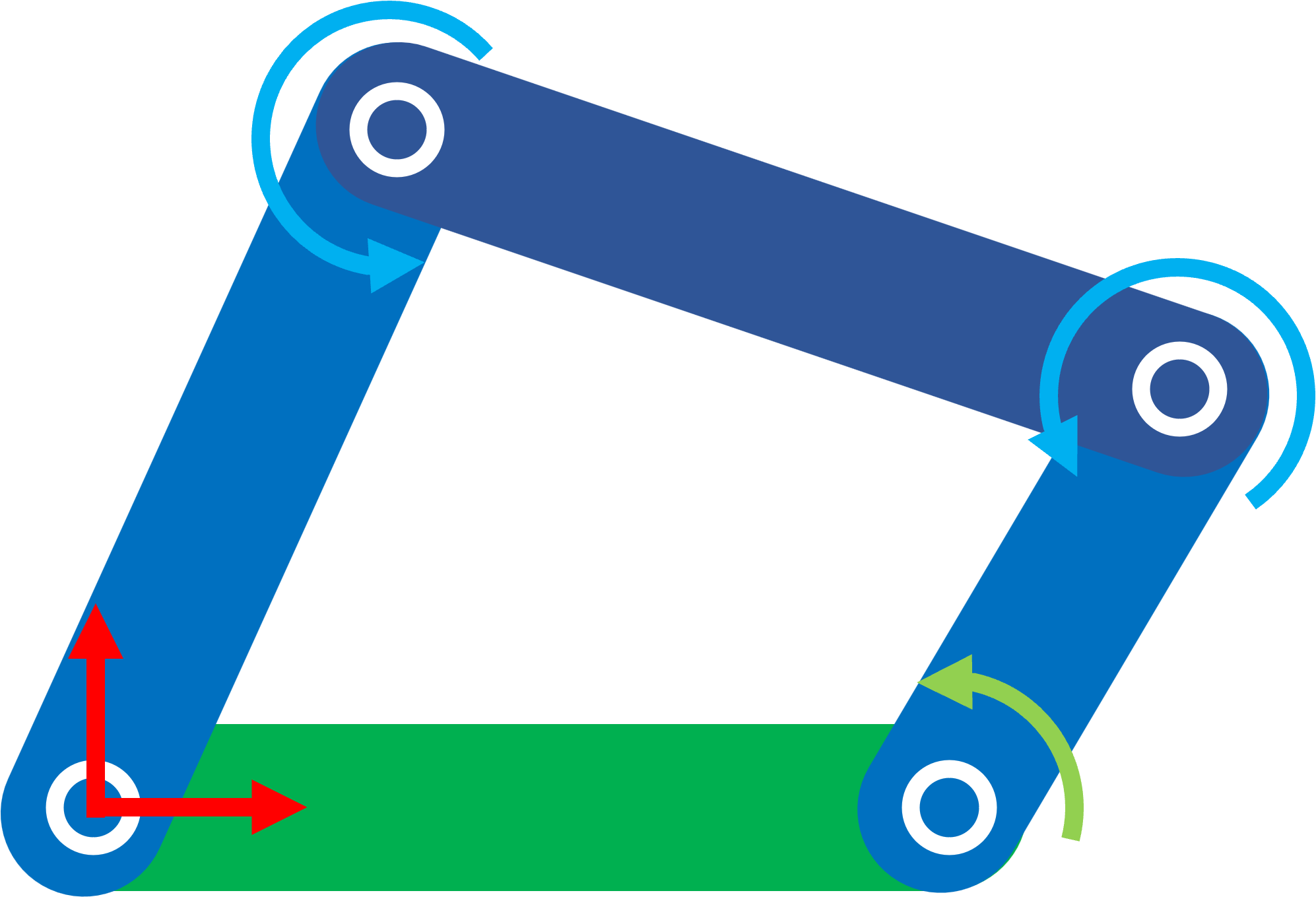 |
4 PinJoints | 3 | 2 | 1 |
 |
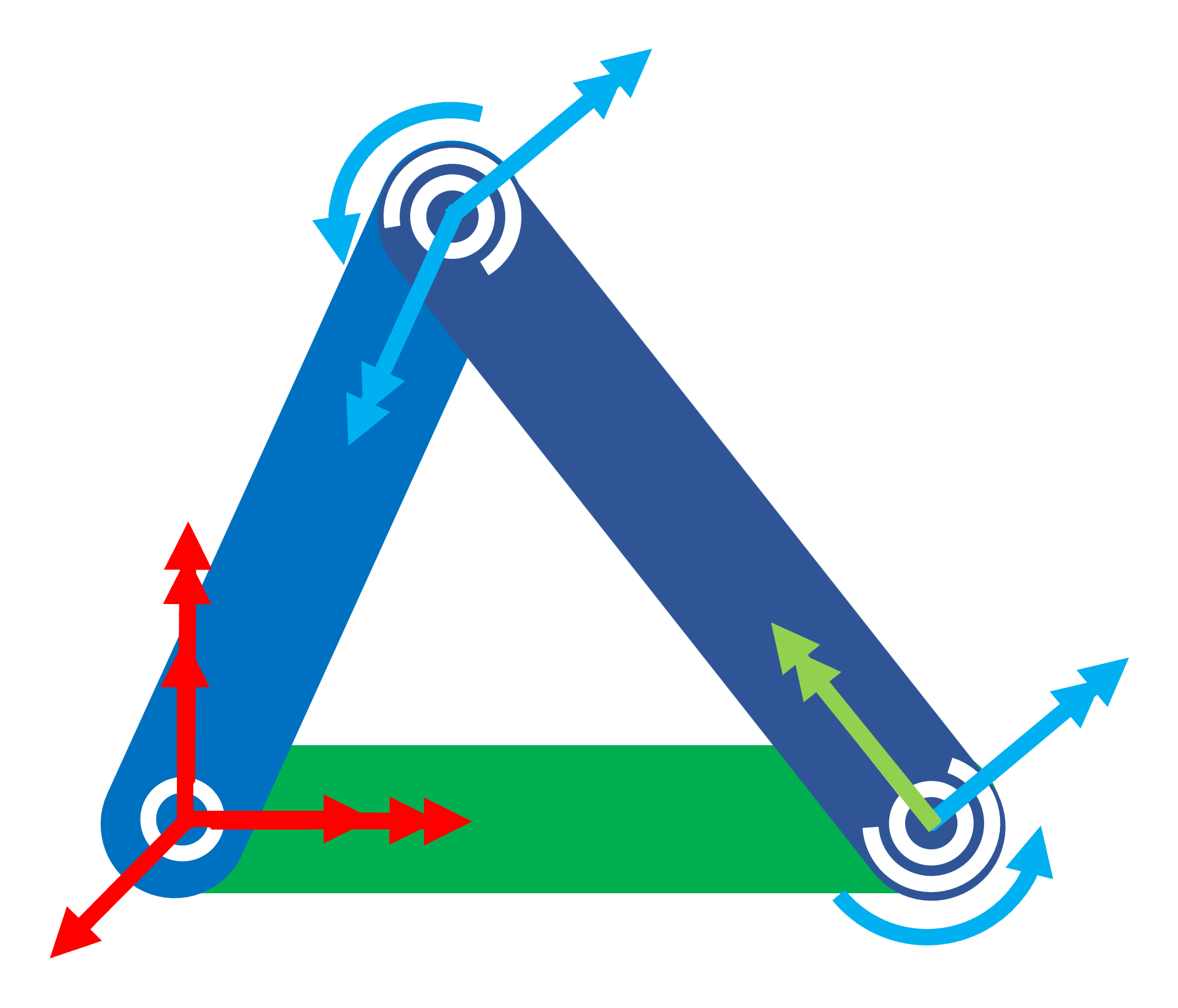
3 PinJoints | 2 | 2 | 0 |
 |
2 SphericalJoints 1 PinJoint | 6 | 5 | 1 |
 |
4 PinJoints 1 PrismaticJoint | 5 | 4 | 1 |
 |
3 PinJoints | 2 | 1 | 1 |
The above list has a few common examples, like the four bar linkage. Other examples mainly test a certain aspect. The three bar linkage is an example, where the entire system is constrained. As for the umbrella you have two kinematic loops which, are dependent on each other in the sense that they have to be exactly the same. So this test will show also how well some terms will drop out. In this case it would also be good to rotate one of the arms around the center axis to make the problem 3D. As for the last example you just have a completely redundant link.
Solution and implementation
Now this is actually the most promising part of this post, at least should be. What we know is that the closing joint adds constraints, which is equal to 6 - #DoF (e.g. PinJoint gives 5) constraints. However some of these are redundant, either because they are simply 0, or because they are the same a combination of one or more other constraints.
Overall I would propose the following solution. Which gathers the constraints closing the kinematic loop from the joints themselves. After which it filters out the active constraints which are then given to the KanesMethod. Here is a bit more elaboration on the points:
- In the
Jointclass it is detected whether a joint would for a loop by trying:parent.frame._dict_list(child.frame, 0) - Assuming it indeed creates a loop, the normal procedure is not followed, instead it does the following:
- The generalized coordinates
qand speedsuare saved within the joint attributes as unused - All configuration constraints are computed, e.g. the
PinJointwould get 5 configuration constraints - These configuration constraints are differentiated to time to get the velocity constraints
- The generalized coordinates
- In the
JointsMethodthe following steps can be taken:- Gather the
q,u,constraints, etc. - Take jacobian of the
velocity_constraintsto the usedu - The rank of
Ushould be equal to the number of active constraints - With this information compute only the active constraints and also split the used
qanduin dependent and independent - This information can then be given to the
KanesMethodwhich will form the equation of motion
- Gather the
Example
Here is some math of how this last part would look like in the JointsMethod with the double link example (last one from the table). From the joint it will get the following information:
\(\vec{q}_{used}=\begin{bmatrix}q_1\\q_2\end{bmatrix}\), \(\vec{q}_{unused}=\begin{bmatrix}q_3\end{bmatrix}\), \(\vec{u}_{used}=\begin{bmatrix}u_1\\u_2\end{bmatrix}\), \(\vec{u}_{unused}=\begin{bmatrix}u_3\end{bmatrix}\)
\(\vec{f}_h=\begin{bmatrix}L \sin{\left(q_{2} \right)}\\L \left(\cos{\left(q_{2} \right)} + 1\right)\\0\\0\\0\end{bmatrix}\)
\(\dot{\vec{f}}_h=\begin{bmatrix}L u_{2} \cos{\left(q_{2} \right)}\\- L u_{2} \sin{\left(q_{2} \right)}\\0\\0\\0\end{bmatrix}\)
For finding the active constraints we first rewrite \(\dot{\vec{f}}_h=M_{hd}\cdot\vec{u}_{used} + g_{hd}\) with \(M_{hd}\) being the jacobian of \(\dot{\vec{f}}_h\) with respect to \(\vec{u}_{used}\):
\(M_{hd}=\begin{bmatrix}0 & L \cos{\left(q_{2} \right)}\\0 & - L \sin{\left(q_{2} \right)}\\0 & 0\\0 & 0\\0 & 0\end{bmatrix}\)
\(g_{hd}=\begin{bmatrix}0\\0\\0\\0\\0\end{bmatrix}\)
LUdecomposition of \(\dot{\vec{f}}_h\) gives:
\(L=\begin{bmatrix}1 & 0 & 0 & 0 & 0\\- \tan{\left(q_{2} \right)} & 1 & 0 & 0 & 0\\0 & 0 & 1 & 0 & 0\\0 & 0 & 0 & 1 & 0\\0 & 0 & 0 & 0 & 1\end{bmatrix}\)
\(U=\begin{bmatrix}0 & L \cos{\left(q_{2} \right)}\\0 & 0\\0 & 0\\0 & 0\\0 & 0\end{bmatrix}\)
As you can clearly see \(rank(U)=1\), so there is one active constraint. Which means that we can use the following equation for the active constraints: L[:rank(U), :] * U * u + g_hd[:rank(U), :]:
\(\begin{bmatrix}1 & 0 & 0 & 0 & 0\end{bmatrix}\cdot\begin{bmatrix}0 & L \cos{\left(q_{2} \right)}\\0 & 0\\0 & 0\\0 & 0\\0 & 0\end{bmatrix}\cdot\begin{bmatrix}u_1\\u_2\end{bmatrix}+\begin{bmatrix}0\end{bmatrix}=\begin{bmatrix}L u_{2} \cos{\left(q_{2} \right)}\end{bmatrix}\)
Note that it should also be possible in this method to immediately solve the problem for the dependent \(\vec{u}\), partially reusing the computed \(L\) and \(U\).
At last the dependent \(\vec{q}\) and \(\vec{u}\) are chosen, using find_dynamicsymbols, and the results are passed on to the KanesMethod.
Some more comments
First of there are still some variations possible on this method. The first part, which determines the constraints in the Joint classes themselves and gathers them in JointsMethod, I think is quite solid and should work. The second part of processing these gathered constraints I see multiple options:
- Generally it would be good to check if some papers provide methods to solve this problem or/and how other physics engines solve it. Would maybe also change the first part if this gives comprising results.
- Use another method of
LUdecomposition, which is more efficient. Sympy has multiple variant on this. - Possibly integrate the part of handling more constraints into the
KanesMethod, so it is also possible to reuse the computedLandU. - If the choice is made to keep it in the
JointMethodthan it would be better to use elementary row operations to determine the active constraints.
Final notes
Thank you for reading this longer than anticipated post if you have any suggestions or questions feel free to use the comments section. Next week I hope to make a post about what issues, PRs, etc. I’ll be working.
Comments
Timo
Something that should also be kept in mind is that the end solution should also be ready for future features around for example adding nonholonomic constraints. Besides this the user should also be able to choose the (in)dependent generalized coordinates. Overall it is important to also think here a bit more about the user API.
Leave a Comment